Find the Fundamental Set of Solutions of the Reduced Equation
The time has finally come to define "nice enough". We've been using this term throughout the last few sections to describe those solutions that could be used to form a general solution and it is now time to officially define it.
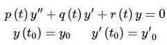
First, because everything that we're going to be doing here only requires linear and homogeneous we won't require constant coefficients in our differential equation. So, let's start with the following IVP.
 ...(1)
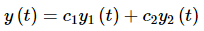
Let's also suppose that we have already found two solutions to this differential equation, y1(t) and y2(t). We know from the Principle of Superposition that
 ...(2)
will also be a solution to the differential equation. What we want to know is whether or not it will be a general solution. In order for (2) to be considered a general solution it must satisfy the general initial conditions in (1).
This will also imply that any solution to the differential equation can be written in this form.
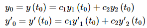
So, let's see if we can find constants that will satisfy these conditions. First differentiate (2) and plug in the initial conditions.
 ...(3)
Since we are assuming that we've already got the two solutions everything in this system is technically known and so this is a system that can be solved for c1 and c2. This can be done in general using Cramer's Rule. Using Cramer's Rule gives the following solution.
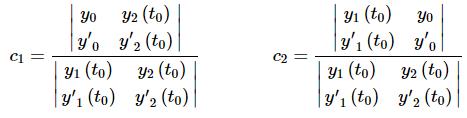 ...(4)
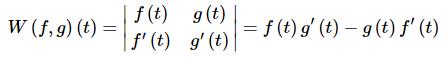
where,
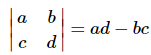
is the determinant of a 2x2 matrix. If you don't know about determinants that is okay, just use the formula that we've provided above.
Now, (4) will give the solution to the system (3). Note that in practice we generally don't use Cramer's Rule to solve systems, we just proceed in a straightforward manner and solve the system using basic algebra techniques. So, why did we use Cramer's Rule here then?
We used Cramer's Rule because we can use (4) to develop a condition that will allow us to determine when we can solve for the constants. All three (yes three, the denominators are the same!) of the quantities in (4) are just numbers and the only thing that will prevent us from actually getting a solution will be when the denominator is zero.
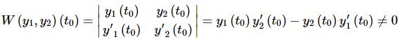
The quantity in the denominator is called the Wronskian and is denoted as
When it is clear what the functions and/or t are we often just denote the Wronskian by W.
Let's recall what we were after here. We wanted to determine when two solutions to.(1)
would be nice enough to form a general solution. The two solutions will form a general solution to (1) if they satisfy the general initial conditions given in (1) and we can see from Cramer's Rule that they will satisfy the initial conditions provided the Wronskian isn't zero. Or,
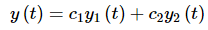
So, suppose that y1(t) and y2(t) are two solutions to (1) and that W(y1,y2)(t)≠0. Then the two solutions are called a fundamental set of solutions and the general solution to (1) is
We know now what "nice enough" means. Two solutions are "nice enough" if they are a fundamental set of solutions.
So, let's check one of the claims that we made in a previous section. We'll leave the other two to you to check if you'd like to.
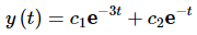
Example 1: Back in the complex root section we made the claim that

were a fundamental set of solutions. Prove that they in fact are.
Solution:So, to prove this we will need to take the Wronskian for these two solutions and show that it isn't zero.
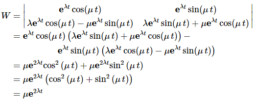
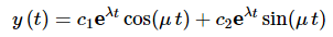
Now, the exponential will never be zero and μ≠0 (if it were we wouldn't have complex roots!) and so W≠0. Therefore, these two solutions are in fact a fundamental set of solutions and so the general solution in this case is.
Example 2: In the first example that we worked in the Reduction of Order section we found a second solution to
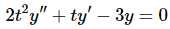
Show that this second solution, along with the given solution, form a fundamental set of solutions for the differential equation.
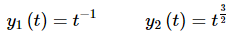
Solution:The two solutions from that example are
Let's compute the Wronskian of these two solutions.
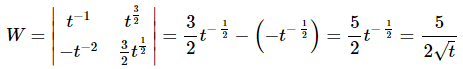
So, the Wronskian will never be zero. Note that we can't plug t = 0 into the Wronskian. This would be a problem in finding the constants in the general solution, except that we also can't plug t = 0 into the solution either and so this isn't the problem that it might appear to be.
So, since the Wronskian isn't zero for any t the two solutions form a fundamental set of solutions and the general solution is
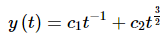
as we claimed in that example.
To this point we've found a set of solutions then we've claimed that they are in fact a fundamental set of solutions. Of course, you can now verify all those claims that we've made, however this does bring up a question. How do we know that for a given differential equation a set of fundamental solutions will exist? The following theorem answers this question.
Theorem
Consider the differential equation
y′′+p(t)y′+q(t)y=0
where p(t) and q(t) are continuous functions on some interval I. Choose t0 to be any point in the interval I. Let y1(t) be a solution to the differential equation that satisfies the initial conditions.
y(t0)=1y′(t0)=0
Let y2(t)
be a solution to the differential equation that satisfies the initial conditions.
y(t0=0y′(t0)=1
Then y1(t) and y2(t) form a fundamental set of solutions for the differential equation.
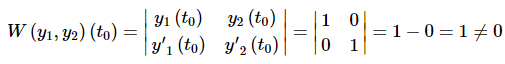
It is easy enough to show that these two solutions form a fundamental set of solutions. Just compute the Wronskian.
So, fundamental sets of solutions will exist provided we can solve the two IVP's given in the theorem.
Example 3: Use the theorem to find a fundamental set of solutions for
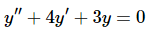
using t0=0.
Solution:Using the techniques from the first part of this chapter we can find the two solutions that we've been using to this point.
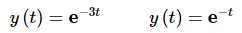
These do form a fundamental set of solutions as we can easily verify. However, they are NOT the set that will be given by the theorem. Neither of these solutions will satisfy either of the two sets of initial conditions given in the theorem. We will have to use these to find the fundamental set of solutions that is given by the theorem.
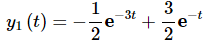
We know that the following is also a solution to the differential equation.
So, let's apply the first set of initial conditions and see if we can find constants that will work.
We'll leave it to you to verify that we get the following solution upon doing this.
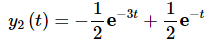
Likewise, if we apply the second set of initial conditions,
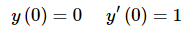
we will get
According to the theorem these should form a fundament set of solutions. This is easy enough to check.
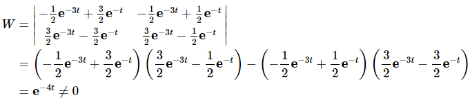
So, we got a completely different set of fundamental solutions from the theorem than what we've been using up to this point. This is not a problem. There are an infinite number of pairs of functions that we could use as a fundamental set of solutions for this problem.
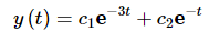
So, which set of fundamental solutions should we use? Well, if we use the ones that we originally found, the general solution would be,
Whereas, if we used the set from the theorem the general solution would be,
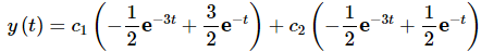
This would not be very fun to work with when it came to determining the coefficients to satisfy a general set of initial conditions.
So, which set of fundamental solutions should we use? We should always try to use the set that is the most convenient to use for a given problem.
More on the Wronskian
In the previous section we introduced the Wronskian to help us determine whether two solutions were a fundamental set of solutions. In this section we will look at another application of the Wronskian as well as an alternate method of computing the Wronskian.
Let's start with the application. We need to introduce a couple of new concepts first.
Given two non-zero functions f(x) and g (x) write down the following equation.
Notice that c = 0 and k = 0 will make (1) true for all x regardless of the functions that we use.
Now, if we can find non-zero constants c and k for which (1) will also be true for all x then we call the two functions linearly dependent. On the other hand if the only two constantsfor which (1) is true are c = 0 and k = 0 then we call the functions linearly independent.
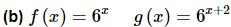
Example 1: Determine if the following sets of functions are linearly dependent or linearly independent.

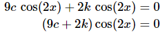
Solution:We'll start by writing down (1) for these two functions.

We need to determine if we can find non-zero constants c and k that will make this true for all x or if c = 0 and k = 0 are the only constants that will make this true for all x. This is often a fairly difficult process. The process can be simplified with a good intuition for this kind of thing, but that's hard to come by, especially if you haven't done many of these kinds of problems.
In this case the problem can be simplified by recalling
Using this fact our equation becomes.
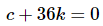
With this simplification we can see that this will be zero for any pair of constants c and k that satisfy
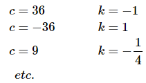
Among the possible pairs on constants that we could use are the following pairs.
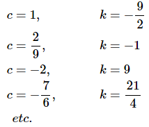
As we're sure you can see there are literally thousands of possible pairs and they can be made as "simple" or as "complicated" as you want them to be.
So, we've managed to find a pair of non-zero constants that will make the equation true for all x and so the two functions are linearly dependent.
Ans:As with the last part, we'll start by writing down (1) for these functions.
In this case there isn't any quick and simple formula to write one of the functions in terms of the other as we did in the first part. So, we're just going to have to see if we can find constants. We'll start by noticing that if the original equation is true, then if we differentiate everything we get a new equation that must also be true. In other words, we've got the following system of two equations in two unknowns.
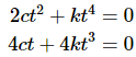
We can solve this system for c and k and see what we get. We'll start by solving the second equation for c.

Now, plug this into the first equation.
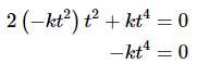
Recall that we are after constants that will make this true for all t. The only way that this will ever be zero for all t is if k = 0! So, if k = 0 we must also have c = 0.
Therefore, we've shown that the only way that
will be true for all t is to require that c = 0 and k = 0. The two functions therefore, are linearly independent.
As we saw in the previous examples determining whether two functions are linearly independent or linearly dependent can be a fairly involved process. This is where the Wronskian can help.
Fact
Given two functions f(x) and g(x) that are differentiable on some interval I.
1. If W(f,g)(x0)≠0 for some x0 in I, then f(x) and g(x) are linearly independent on the interval I.
2. If f(x) and g(x) are linearly dependent on I then W(f,g)(x)=0 for all x in the interval I.
Be very careful with this fact. It DOES NOT say that if W(f,g)(x)=0 then f(x) and g(x) are linearly dependent! In fact, it is possible for two linearly independent functions to have a zero Wronskian!
This fact is used to quickly identify linearly independent functions and functions that are liable to be linearly dependent.
Example 2: Verify the fact using the functions from the previous example.

Solution: In this case if we compute the Wronskian of the two functions we should get zero since we have already determined that these functions are linearly dependent.
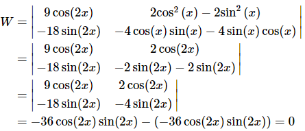
So, we get zero as we should have. Notice the heavy use of trig formulas to simplify the work!
Solution:Here we know that the two functions are linearly independent and so we should get a non-zero Wronskian.
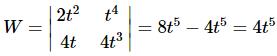
The Wronskian is non-zero as we expected provided t≠0. This is not a problem. As long as the Wronskian is not identically zero for all t we are okay.
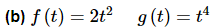
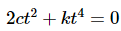
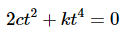
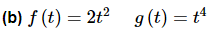
Example 3: Determine if the following functions are linearly dependent or linearly independent.
Solution: 
Now that we have the Wronskian to use here let's first check that. If its non-zero then we will know that the two functions are linearly independent and if its zero then we can be pretty sure that they are linearly dependent.
So, by the fact these two functions are linearly independent. Much easier this time around!
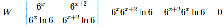
We'll do the same thing here as we did in the first part. Recall that
Now compute the Wronskian.
Now, this does not say that the two functions are linearly dependent! However, we can guess that they probably are linearly dependent. To prove that they are in fact linearly dependent we'll need to write down (1) and see if we can find non-zero c and k that will make it true for all x.
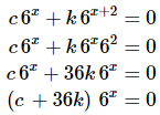
So, it looks like we could use any constants that satisfy
to make this zero for all x. In particular we could use
We have non-zero constants that will make the equation true for all x. Therefore, the functions are linearly dependent.
Before proceeding to the next topic in this section let's talk a little more about linearly independent and linearly dependent functions. Let's start off by assuming that f(x) and g(x) are linearly dependent. So, that means there are non-zero constants c and k so that
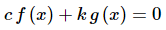
is true for all x.
Now, we can solve this in either of the following two ways.
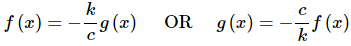
Note that this can be done because we know that cc and kk are non-zero and hence the divisions can be done without worrying about division by zero.
So, this means that two linearly dependent functions can be written in such a way that one is nothing more than a constants time the other. Go back and look at both of the sets of linearly dependent functions that we wrote down and you will see that this is true for both of them.
Two functions that are linearly independent can't be written in this manner and so we can't get from one to the other simply by multiplying by a constant.
Next, we don't want to leave you with the impression that linear independence and linear dependence is only for two functions. We can easily extend the idea to as many functions as we'd like.
Let's suppose that we have nn non-zero functions, f1(x), f2(x),…, fn(x). Write down the following equation.

If we can find constants c1, c2, …, cn with at least two non-zero so that (2) is true for all x then we call the functions linearly dependent. If, on the other hand, the only constants that make (2) true for x are c1=0, c2=0, …, cn=0 then we call the functions linearly independent.
Note that unlike the two function case we can have some of the constants be zero and still have the functions be linearly dependent.
In this case just what does it mean for the functions to be linearly dependent? Well, let's suppose that they are. So, this means that we can find constants, with at least two non zero so that (2) is true for all x. For the sake of argument let's suppose that c1 is one of the non-zero constants. This means that we can do the following.
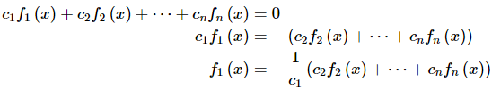
In other words, if the functions are linearly dependent then we can write at least one of them in terms of the other functions.
Okay, let's move on to the other topic of this section. There is an alternate method of computing the Wronskian. The following theorem gives this alternate method.
Abel's Theorem
If y1(t) and y2(t) are two solutions to
y′′+p(t)y′+q(t)y=0
then the Wronskian of the two solutions is
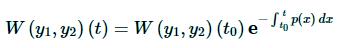
for some t0.
Because we don't know the Wronskian and we don't know t0 this won't do us a lot of good apparently. However, we can rewrite this as
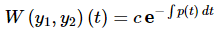
where the original Wronskian sitting in front of the exponential is absorbed into the
c and the evaluation of the integral at t0 will put a constant in the exponential that can also be brought out and absorbed into the constant c. If you don't recall how to do this go back and take a look at the linear, first order differential equation section as we did something similar there.
With this rewrite we can compute the Wronskian up to a multiplicative constant, which isn't too bad. Notice as well that we don't actually need the two solutions to do this. All we need is the coefficient of the first derivative from the differential equation (provided the coefficient of the second derivative is one of course…).
Let's take a look at a quick example of this.
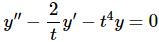
Example 4: Without solving, determine the Wronskian of two solutions to the following differential equation.
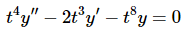
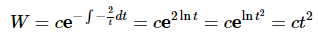
Solution:The first thing that we need to do is divide the differential equation by the coefficient of the second derivative as that needs to be a one. This gives us
Now, using (3) the Wronskian is
Find the Fundamental Set of Solutions of the Reduced Equation
Source: https://edurev.in/studytube/Fundamental-Sets-of-Solutions/3ef80e4f-aedc-4490-8d57-56a4abfc75f9_t